Python for Data Analysis and Visualization

---

     

A Tufts University Data Lab Workshop
Written by Uku-Kaspar Uustalu

Python resources: go.tufts.edu/python
Questions: datalab-support@elist.tufts.edu
Feedback: uku-kaspar.uustalu@tufts.edu

---

Importing Libraries

import numpy as np
import pandas as pd
import matplotlib.pyplot as plt
import seaborn as sns

---------------------------------------------------------------------------
ModuleNotFoundError                       Traceback (most recent call last)
Cell In[1], line 3
      1 import numpy as np
      2 import pandas as pd
----> 3 import matplotlib.pyplot as plt
      4 import seaborn as sns

ModuleNotFoundError: No module named 'matplotlib'

---

Quick Overview of Matplotlib

Matplotlib works in a layered fashion. First you define your plot using plt.plot(x, y, ...), then you can use additional plt methods to add more layers to your plot or modify its appearance. Finally, you use plt.show() to show the plot or plt.savefig() to save it to an external file. Let’s see how Matplotlib works in practice by creating some trigonometric plots.

x = np.linspace(0, 2 * np.pi, num = 20)
y = np.sin(x)

plt.plot(x, y)
plt.show()

plt.plot() takes additional arguments that modify the appearance of the plot. See the documentation for details: https://matplotlib.org/api/_as_gen/matplotlib.pyplot.plot.html

# we can specify the style of the plot using named arguments
plt.plot(x, y, color = 'red', linestyle = '--', marker = 'o')
plt.show()

# or we could use a shorthand string
plt.plot(x, y, 'r--o')
plt.show()

We can easily add additional layers and stylistic elements to the plot.

plt.plot(x, y, 'r--o')
plt.plot(x, np.cos(x), 'b-*')
plt.title('Sin and Cos')
plt.xlabel('x')
plt.ylabel('y')
plt.legend(['sin', 'cos'])
plt.show()

Note that if we only supply one array as an input to plt.plot(), it uses the values of the array as y values and uses the indices of the array as x values.

plt.plot([2, 3, 6, 4, 8, 9, 5, 7, 1])
plt.show()

If we want to create a figure with several subplots, we can use plt.subplots() to create a grid of subplots. It takes the dimensions of the subplot grid as input plt.subplots(rows, columns) and returns tow objects. The first is a figure object and the second is a NumPy array containing the subplots. In Matplotlib, subplots are often called axes.

# create a more fine-grained array to work with
a = np.linspace(0, 2 * np.pi, num = 100)

# create a two-by-two grid for our subplots
fig, ax = plt.subplots(2, 2)

# create subplots
ax[0, 0].plot(a, np.sin(a))     # upper-left
ax[0, 1].plot(a, np.cos(a))     # upper-right
ax[1, 0].plot(a, np.tan(a))     # bottom-left
ax[1, 1].plot(a, -a)            # bottom-right

# show figure
plt.show()

A more MATLAB-esque way of creating subplots would be to use the alternative plt.subplot() method. Using this method, you can define subplot using a three-number combination plt.subplot(rows, columns, index). The indexes of the subplots defined using this method increase in row-major order and, in true MATLAB fashion, begin with one.

plt.subplot(2, 2, 1)    # upper-left
plt.plot(a, np.sin(a))
plt.subplot(2, 2, 2)    # upper-right
plt.plot(a, np.cos(a))
plt.subplot(2, 2, 3)    # bottom-left
plt.plot(a, np.tan(a))
plt.subplot(2, 2, 4)    # bottom-right
plt.plot(a, -a)
plt.show()

---

Working with Messy Data

grades = pd.read_csv('data/grades.csv')

grades

	Name	Exam 1	exam2	Exam_3	exam4
0	John Smith	98	94	95	86
1	Mary Johnson	89	92	96	82
2	Robert Williams	88	72	absent	91
3	Jennifer Jones	92	excused	94	99
4	Linda Wilson	84	92	89	94

print(grades)

              Name  Exam 1    exam2  Exam_3  exam4
0       John Smith      98       94      95     86
1     Mary Johnson      89       92      96     82
2  Robert Williams      88       72  absent     91
3   Jennifer Jones      92  excused      94     99
4     Linda Wilson      84       92      89     94

Cleaning Column Names

grades.rename(str.lower, axis = 'columns')

	name	exam 1	exam2	exam_3	exam4
0	John Smith	98	94	95	86
1	Mary Johnson	89	92	96	82
2	Robert Williams	88	72	absent	91
3	Jennifer Jones	92	excused	94	99
4	Linda Wilson	84	92	89	94

grades

	Name	Exam 1	exam2	Exam_3	exam4
0	John Smith	98	94	95	86
1	Mary Johnson	89	92	96	82
2	Robert Williams	88	72	absent	91
3	Jennifer Jones	92	excused	94	99
4	Linda Wilson	84	92	89	94

grades = grades.rename(str.lower, axis = 'columns')

grades

	name	exam 1	exam2	exam_3	exam4
0	John Smith	98	94	95	86
1	Mary Johnson	89	92	96	82
2	Robert Williams	88	72	absent	91
3	Jennifer Jones	92	excused	94	99
4	Linda Wilson	84	92	89	94

grades.rename(columns = {'exam 1': 'exam1', 'exam_3': 'exam3'}, inplace = True)

grades

	name	exam1	exam2	exam3	exam4
0	John Smith	98	94	95	86
1	Mary Johnson	89	92	96	82
2	Robert Williams	88	72	absent	91
3	Jennifer Jones	92	excused	94	99
4	Linda Wilson	84	92	89	94

Indexing and Datatypes

grades.dtypes

name     object
exam1     int64
exam2    object
exam3    object
exam4     int64
dtype: object

grades['name']

0         John Smith
1       Mary Johnson
2    Robert Williams
3     Jennifer Jones
4       Linda Wilson
Name: name, dtype: object

grades.name

0         John Smith
1       Mary Johnson
2    Robert Williams
3     Jennifer Jones
4       Linda Wilson
Name: name, dtype: object

grades[['name']]

	name
0	John Smith
1	Mary Johnson
2	Robert Williams
3	Jennifer Jones
4	Linda Wilson

grades['name'][0]

'John Smith'

grades['name'][1]

'Mary Johnson'

grades.name[1]

'Mary Johnson'

grades['exam1'][1]

89

grades.exam2[1]

'92'

grades['exam3'][1]

'96'

grades.exam4[1]

82

grades

	name	exam1	exam2	exam3	exam4
0	John Smith	98	94	95	86
1	Mary Johnson	89	92	96	82
2	Robert Williams	88	72	absent	91
3	Jennifer Jones	92	excused	94	99
4	Linda Wilson	84	92	89	94

print(type(grades['exam3'][0]))
print(type(grades['exam3'][1]))
print(type(grades['exam3'][2]))

<class 'str'>
<class 'str'>
<class 'str'>

Assigning Values and Working with Missing Data

grades['exam3'][2] = 0

C:\Users\bzhou01\AppData\Local\Temp\ipykernel_22684\2777045509.py:1: SettingWithCopyWarning: 
A value is trying to be set on a copy of a slice from a DataFrame

See the caveats in the documentation: https://pandas.pydata.org/pandas-docs/stable/user_guide/indexing.html#returning-a-view-versus-a-copy
  grades['exam3'][2] = 0

Oh no, a really scary warning! What is happening?

Because Python uses something called pass-by-object-reference and does a lot of optimization in the background, the end user (that is you) has little to no control over whether thay are referencing the original object or a copy. This warning is just Pandas letting us know that when using chained indexing to write a value, the behaviour is undefined, meaning that pandas cannot be sure wheter you are are writing to the original data frame or a temporary copy.

To learn more: https://pandas.pydata.org/pandas-docs/stable/user_guide/indexing.html#returning-a-view-versus-a-copy

grades

	name	exam1	exam2	exam3	exam4
0	John Smith	98	94	95	86
1	Mary Johnson	89	92	96	82
2	Robert Williams	88	72	0	91
3	Jennifer Jones	92	excused	94	99
4	Linda Wilson	84	92	89	94

Phew, this time we got lucky. However, with a differet data frame the same approach might actually write the changes to a temporary copy and leave the original data frame unchanged. Chained indexing is dangerous and you should avoid using it to write values. What should we use instead?

There are a lot of options: https://pandas.pydata.org/pandas-docs/stable/user_guide/indexing.html

• To write a singe value, use .at[row, column]

• To write a range of values (or a single value), use .loc[row(s), column(s)]

Note that .at and .loc use row and column labels. The numbers 0, 1, 2, 3, and 4 that we see in front of the rows are actually row labels. By default, row labels match row indexes in pandas. However, quite often you will work with rows that have actual labels. Sometimes those labels might be numeric and resemble indexes, which leads to confusion and error. Hence, if you want to make sure you are using indexes, not labels, use .iat and .iloc instead.

grades.at[2, 'exam3']

0

grades.loc[3, 'exam2'] = np.NaN

grades

	name	exam1	exam2	exam3	exam4
0	John Smith	98	94	95	86
1	Mary Johnson	89	92	96	82
2	Robert Williams	88	72	0	91
3	Jennifer Jones	92	NaN	94	99
4	Linda Wilson	84	92	89	94

grades.dtypes

name     object
exam1     int64
exam2    object
exam3    object
exam4     int64
dtype: object

grades['exam2'][0]

'94'

grades.exam3[0]

'95'

grades['exam2'] = pd.to_numeric(grades['exam2'])
grades['exam3'] = pd.to_numeric(grades.exam3)

grades

	name	exam1	exam2	exam3	exam4
0	John Smith	98	94.0	95	86
1	Mary Johnson	89	92.0	96	82
2	Robert Williams	88	72.0	0	91
3	Jennifer Jones	92	NaN	94	99
4	Linda Wilson	84	92.0	89	94

grades.dtypes

name      object
exam1      int64
exam2    float64
exam3      int64
exam4      int64
dtype: object

Aggregating Data

grades['sum'] = grades['exam1'] + grades['exam2'] + grades['exam3'] + grades['exam4']

grades

	name	exam1	exam2	exam3	exam4	sum
0	John Smith	98	94.0	95	86	373.0
1	Mary Johnson	89	92.0	96	82	359.0
2	Robert Williams	88	72.0	0	91	251.0
3	Jennifer Jones	92	NaN	94	99	NaN
4	Linda Wilson	84	92.0	89	94	359.0

grades.drop('sum', axis = 'columns', inplace = True)

grades

	name	exam1	exam2	exam3	exam4
0	John Smith	98	94.0	95	86
1	Mary Johnson	89	92.0	96	82
2	Robert Williams	88	72.0	0	91
3	Jennifer Jones	92	NaN	94	99
4	Linda Wilson	84	92.0	89	94

grades['sum'] = grades.sum(axis = 'columns')

---------------------------------------------------------------------------
TypeError                                 Traceback (most recent call last)
Cell In[77], line 1
----> 1 grades['sum'] = grades.sum(axis = 'columns')

File C:\JumboConda\lib\site-packages\pandas\core\frame.py:11312, in DataFrame.sum(self, axis, skipna, numeric_only, min_count, **kwargs)
  11303 @doc(make_doc("sum", ndim=2))
  11304 def sum(
  11305     self,
   (...)
  11310     **kwargs,
  11311 ):
> 11312     result = super().sum(axis, skipna, numeric_only, min_count, **kwargs)
  11313     return result.__finalize__(self, method="sum")

File C:\JumboConda\lib\site-packages\pandas\core\generic.py:12078, in NDFrame.sum(self, axis, skipna, numeric_only, min_count, **kwargs)
  12070 def sum(
  12071     self,
  12072     axis: Axis | None = 0,
   (...)
  12076     **kwargs,
  12077 ):
> 12078     return self._min_count_stat_function(
  12079         "sum", nanops.nansum, axis, skipna, numeric_only, min_count, **kwargs
  12080     )

File C:\JumboConda\lib\site-packages\pandas\core\generic.py:12061, in NDFrame._min_count_stat_function(self, name, func, axis, skipna, numeric_only, min_count, **kwargs)
  12058 elif axis is lib.no_default:
  12059     axis = 0
> 12061 return self._reduce(
  12062     func,
  12063     name=name,
  12064     axis=axis,
  12065     skipna=skipna,
  12066     numeric_only=numeric_only,
  12067     min_count=min_count,
  12068 )

File C:\JumboConda\lib\site-packages\pandas\core\frame.py:11204, in DataFrame._reduce(self, op, name, axis, skipna, numeric_only, filter_type, **kwds)
  11200     df = df.T
  11202 # After possibly _get_data and transposing, we are now in the
  11203 #  simple case where we can use BlockManager.reduce
> 11204 res = df._mgr.reduce(blk_func)
  11205 out = df._constructor_from_mgr(res, axes=res.axes).iloc[0]
  11206 if out_dtype is not None and out.dtype != "boolean":

File C:\JumboConda\lib\site-packages\pandas\core\internals\managers.py:1459, in BlockManager.reduce(self, func)
   1457 res_blocks: list[Block] = []
   1458 for blk in self.blocks:
-> 1459     nbs = blk.reduce(func)
   1460     res_blocks.extend(nbs)
   1462 index = Index([None])  # placeholder

File C:\JumboConda\lib\site-packages\pandas\core\internals\blocks.py:377, in Block.reduce(self, func)
    371 @final
    372 def reduce(self, func) -> list[Block]:
    373     # We will apply the function and reshape the result into a single-row
    374     #  Block with the same mgr_locs; squeezing will be done at a higher level
    375     assert self.ndim == 2
--> 377     result = func(self.values)
    379     if self.values.ndim == 1:
    380         res_values = result

File C:\JumboConda\lib\site-packages\pandas\core\frame.py:11136, in DataFrame._reduce.<locals>.blk_func(values, axis)
  11134         return np.array([result])
  11135 else:
> 11136     return op(values, axis=axis, skipna=skipna, **kwds)

File C:\JumboConda\lib\site-packages\pandas\core\nanops.py:85, in disallow.__call__.<locals>._f(*args, **kwargs)
     81     raise TypeError(
     82         f"reduction operation '{f_name}' not allowed for this dtype"
     83     )
     84 try:
---> 85     return f(*args, **kwargs)
     86 except ValueError as e:
     87     # we want to transform an object array
     88     # ValueError message to the more typical TypeError
     89     # e.g. this is normally a disallowed function on
     90     # object arrays that contain strings
     91     if is_object_dtype(args[0]):

File C:\JumboConda\lib\site-packages\pandas\core\nanops.py:404, in _datetimelike_compat.<locals>.new_func(values, axis, skipna, mask, **kwargs)
    401 if datetimelike and mask is None:
    402     mask = isna(values)
--> 404 result = func(values, axis=axis, skipna=skipna, mask=mask, **kwargs)
    406 if datetimelike:
    407     result = _wrap_results(result, orig_values.dtype, fill_value=iNaT)

File C:\JumboConda\lib\site-packages\pandas\core\nanops.py:477, in maybe_operate_rowwise.<locals>.newfunc(values, axis, **kwargs)
    474         results = [func(x, **kwargs) for x in arrs]
    475     return np.array(results)
--> 477 return func(values, axis=axis, **kwargs)

File C:\JumboConda\lib\site-packages\pandas\core\nanops.py:646, in nansum(values, axis, skipna, min_count, mask)
    643 elif dtype.kind == "m":
    644     dtype_sum = np.dtype(np.float64)
--> 646 the_sum = values.sum(axis, dtype=dtype_sum)
    647 the_sum = _maybe_null_out(the_sum, axis, mask, values.shape, min_count=min_count)
    649 return the_sum

File C:\JumboConda\lib\site-packages\numpy\core\_methods.py:49, in _sum(a, axis, dtype, out, keepdims, initial, where)
     47 def _sum(a, axis=None, dtype=None, out=None, keepdims=False,
     48          initial=_NoValue, where=True):
---> 49     return umr_sum(a, axis, dtype, out, keepdims, initial, where)

TypeError: can only concatenate str (not "int") to str

grades

	name	exam1	exam2	exam3	exam4
0	John Smith	98	94.0	95	86
1	Mary Johnson	89	92.0	96	82
2	Robert Williams	88	72.0	0	91
3	Jennifer Jones	92	NaN	94	99
4	Linda Wilson	84	92.0	89	94

---

A Better Way of Working with Messy Data

del grades

grades = pd.read_csv('data/grades.csv', na_values = 'excused')
grades

	Name	Exam 1	exam2	Exam_3	exam4
0	John Smith	98	94.0	95	86
1	Mary Johnson	89	92.0	96	82
2	Robert Williams	88	72.0	absent	91
3	Jennifer Jones	92	NaN	94	99
4	Linda Wilson	84	92.0	89	94

grades.rename(str.lower, axis = 'columns', inplace = True)
grades.rename(columns = {'exam 1': 'exam1', 'exam_3': 'exam3'}, inplace = True)
grades

	name	exam1	exam2	exam3	exam4
0	John Smith	98	94.0	95	86
1	Mary Johnson	89	92.0	96	82
2	Robert Williams	88	72.0	absent	91
3	Jennifer Jones	92	NaN	94	99
4	Linda Wilson	84	92.0	89	94

grades.dtypes

name      object
exam1      int64
exam2    float64
exam3     object
exam4      int64
dtype: object

grades['exam3'] = pd.to_numeric(grades['exam3'], errors = 'coerce')
grades

	name	exam1	exam2	exam3	exam4
0	John Smith	98	94.0	95.0	86
1	Mary Johnson	89	92.0	96.0	82
2	Robert Williams	88	72.0	NaN	91
3	Jennifer Jones	92	NaN	94.0	99
4	Linda Wilson	84	92.0	89.0	94

grades.dtypes

name      object
exam1      int64
exam2    float64
exam3    float64
exam4      int64
dtype: object

grades['exam3'] = grades['exam3'].fillna(0)
grades['name'][2]

'Robert Williams'

grades['mean'] = grades.mean(axis = 'columns')
grades

---------------------------------------------------------------------------
TypeError                                 Traceback (most recent call last)
Cell In[130], line 1
----> 1 grades['mean'] = grades.mean(axis = 'columns')
      2 grades
      3 grades["name"]

File C:\JumboConda\lib\site-packages\pandas\core\frame.py:11335, in DataFrame.mean(self, axis, skipna, numeric_only, **kwargs)
  11327 @doc(make_doc("mean", ndim=2))
  11328 def mean(
  11329     self,
   (...)
  11333     **kwargs,
  11334 ):
> 11335     result = super().mean(axis, skipna, numeric_only, **kwargs)
  11336     if isinstance(result, Series):
  11337         result = result.__finalize__(self, method="mean")

File C:\JumboConda\lib\site-packages\pandas\core\generic.py:11992, in NDFrame.mean(self, axis, skipna, numeric_only, **kwargs)
  11985 def mean(
  11986     self,
  11987     axis: Axis | None = 0,
   (...)
  11990     **kwargs,
  11991 ) -> Series | float:
> 11992     return self._stat_function(
  11993         "mean", nanops.nanmean, axis, skipna, numeric_only, **kwargs
  11994     )

File C:\JumboConda\lib\site-packages\pandas\core\generic.py:11949, in NDFrame._stat_function(self, name, func, axis, skipna, numeric_only, **kwargs)
  11945 nv.validate_func(name, (), kwargs)
  11947 validate_bool_kwarg(skipna, "skipna", none_allowed=False)
> 11949 return self._reduce(
  11950     func, name=name, axis=axis, skipna=skipna, numeric_only=numeric_only
  11951 )

File C:\JumboConda\lib\site-packages\pandas\core\frame.py:11204, in DataFrame._reduce(self, op, name, axis, skipna, numeric_only, filter_type, **kwds)
  11200     df = df.T
  11202 # After possibly _get_data and transposing, we are now in the
  11203 #  simple case where we can use BlockManager.reduce
> 11204 res = df._mgr.reduce(blk_func)
  11205 out = df._constructor_from_mgr(res, axes=res.axes).iloc[0]
  11206 if out_dtype is not None and out.dtype != "boolean":

File C:\JumboConda\lib\site-packages\pandas\core\internals\managers.py:1459, in BlockManager.reduce(self, func)
   1457 res_blocks: list[Block] = []
   1458 for blk in self.blocks:
-> 1459     nbs = blk.reduce(func)
   1460     res_blocks.extend(nbs)
   1462 index = Index([None])  # placeholder

File C:\JumboConda\lib\site-packages\pandas\core\internals\blocks.py:377, in Block.reduce(self, func)
    371 @final
    372 def reduce(self, func) -> list[Block]:
    373     # We will apply the function and reshape the result into a single-row
    374     #  Block with the same mgr_locs; squeezing will be done at a higher level
    375     assert self.ndim == 2
--> 377     result = func(self.values)
    379     if self.values.ndim == 1:
    380         res_values = result

File C:\JumboConda\lib\site-packages\pandas\core\frame.py:11136, in DataFrame._reduce.<locals>.blk_func(values, axis)
  11134         return np.array([result])
  11135 else:
> 11136     return op(values, axis=axis, skipna=skipna, **kwds)

File C:\JumboConda\lib\site-packages\pandas\core\nanops.py:147, in bottleneck_switch.__call__.<locals>.f(values, axis, skipna, **kwds)
    145         result = alt(values, axis=axis, skipna=skipna, **kwds)
    146 else:
--> 147     result = alt(values, axis=axis, skipna=skipna, **kwds)
    149 return result

File C:\JumboConda\lib\site-packages\pandas\core\nanops.py:404, in _datetimelike_compat.<locals>.new_func(values, axis, skipna, mask, **kwargs)
    401 if datetimelike and mask is None:
    402     mask = isna(values)
--> 404 result = func(values, axis=axis, skipna=skipna, mask=mask, **kwargs)
    406 if datetimelike:
    407     result = _wrap_results(result, orig_values.dtype, fill_value=iNaT)

File C:\JumboConda\lib\site-packages\pandas\core\nanops.py:719, in nanmean(values, axis, skipna, mask)
    716     dtype_count = dtype
    718 count = _get_counts(values.shape, mask, axis, dtype=dtype_count)
--> 719 the_sum = values.sum(axis, dtype=dtype_sum)
    720 the_sum = _ensure_numeric(the_sum)
    722 if axis is not None and getattr(the_sum, "ndim", False):

File C:\JumboConda\lib\site-packages\numpy\core\_methods.py:49, in _sum(a, axis, dtype, out, keepdims, initial, where)
     47 def _sum(a, axis=None, dtype=None, out=None, keepdims=False,
     48          initial=_NoValue, where=True):
---> 49     return umr_sum(a, axis, dtype, out, keepdims, initial, where)

TypeError: can only concatenate str (not "int") to str

grades.loc[:, 'max'] = grades.max(axis = 'columns')
grades.loc['mean'] = grades.mean(axis = 'rows')
grades.loc['max', :] = grades.max(axis = 'rows')
grades

---------------------------------------------------------------------------
TypeError                                 Traceback (most recent call last)
Cell In[87], line 1
----> 1 grades.loc[:, 'max'] = grades.max(axis = 'columns')
      2 grades.loc['mean'] = grades.mean(axis = 'rows')
      3 grades.loc['max', :] = grades.max(axis = 'rows')

File C:\JumboConda\lib\site-packages\pandas\core\frame.py:11298, in DataFrame.max(self, axis, skipna, numeric_only, **kwargs)
  11290 @doc(make_doc("max", ndim=2))
  11291 def max(
  11292     self,
   (...)
  11296     **kwargs,
  11297 ):
> 11298     result = super().max(axis, skipna, numeric_only, **kwargs)
  11299     if isinstance(result, Series):
  11300         result = result.__finalize__(self, method="max")

File C:\JumboConda\lib\site-packages\pandas\core\generic.py:11976, in NDFrame.max(self, axis, skipna, numeric_only, **kwargs)
  11969 def max(
  11970     self,
  11971     axis: Axis | None = 0,
   (...)
  11974     **kwargs,
  11975 ):
> 11976     return self._stat_function(
  11977         "max",
  11978         nanops.nanmax,
  11979         axis,
  11980         skipna,
  11981         numeric_only,
  11982         **kwargs,
  11983     )

File C:\JumboConda\lib\site-packages\pandas\core\generic.py:11949, in NDFrame._stat_function(self, name, func, axis, skipna, numeric_only, **kwargs)
  11945 nv.validate_func(name, (), kwargs)
  11947 validate_bool_kwarg(skipna, "skipna", none_allowed=False)
> 11949 return self._reduce(
  11950     func, name=name, axis=axis, skipna=skipna, numeric_only=numeric_only
  11951 )

File C:\JumboConda\lib\site-packages\pandas\core\frame.py:11204, in DataFrame._reduce(self, op, name, axis, skipna, numeric_only, filter_type, **kwds)
  11200     df = df.T
  11202 # After possibly _get_data and transposing, we are now in the
  11203 #  simple case where we can use BlockManager.reduce
> 11204 res = df._mgr.reduce(blk_func)
  11205 out = df._constructor_from_mgr(res, axes=res.axes).iloc[0]
  11206 if out_dtype is not None and out.dtype != "boolean":

File C:\JumboConda\lib\site-packages\pandas\core\internals\managers.py:1459, in BlockManager.reduce(self, func)
   1457 res_blocks: list[Block] = []
   1458 for blk in self.blocks:
-> 1459     nbs = blk.reduce(func)
   1460     res_blocks.extend(nbs)
   1462 index = Index([None])  # placeholder

File C:\JumboConda\lib\site-packages\pandas\core\internals\blocks.py:377, in Block.reduce(self, func)
    371 @final
    372 def reduce(self, func) -> list[Block]:
    373     # We will apply the function and reshape the result into a single-row
    374     #  Block with the same mgr_locs; squeezing will be done at a higher level
    375     assert self.ndim == 2
--> 377     result = func(self.values)
    379     if self.values.ndim == 1:
    380         res_values = result

File C:\JumboConda\lib\site-packages\pandas\core\frame.py:11136, in DataFrame._reduce.<locals>.blk_func(values, axis)
  11134         return np.array([result])
  11135 else:
> 11136     return op(values, axis=axis, skipna=skipna, **kwds)

File C:\JumboConda\lib\site-packages\pandas\core\nanops.py:147, in bottleneck_switch.__call__.<locals>.f(values, axis, skipna, **kwds)
    145         result = alt(values, axis=axis, skipna=skipna, **kwds)
    146 else:
--> 147     result = alt(values, axis=axis, skipna=skipna, **kwds)
    149 return result

File C:\JumboConda\lib\site-packages\pandas\core\nanops.py:404, in _datetimelike_compat.<locals>.new_func(values, axis, skipna, mask, **kwargs)
    401 if datetimelike and mask is None:
    402     mask = isna(values)
--> 404 result = func(values, axis=axis, skipna=skipna, mask=mask, **kwargs)
    406 if datetimelike:
    407     result = _wrap_results(result, orig_values.dtype, fill_value=iNaT)

File C:\JumboConda\lib\site-packages\pandas\core\nanops.py:1092, in _nanminmax.<locals>.reduction(values, axis, skipna, mask)
   1087     return _na_for_min_count(values, axis)
   1089 values, mask = _get_values(
   1090     values, skipna, fill_value_typ=fill_value_typ, mask=mask
   1091 )
-> 1092 result = getattr(values, meth)(axis)
   1093 result = _maybe_null_out(result, axis, mask, values.shape)
   1094 return result

File C:\JumboConda\lib\site-packages\numpy\core\_methods.py:41, in _amax(a, axis, out, keepdims, initial, where)
     39 def _amax(a, axis=None, out=None, keepdims=False,
     40           initial=_NoValue, where=True):
---> 41     return umr_maximum(a, axis, None, out, keepdims, initial, where)

TypeError: '>=' not supported between instances of 'str' and 'int'

---

Working with Real Data

avocados = pd.read_csv('data/avocado.csv')

avocados

	date	average_price	total_volume	4046	4225	4770	total_bags	small_bags	large_bags	xlarge_bags	type	year	geography
0	2015-01-04	1.22	40873.28	2819.50	28287.42	49.90	9716.46	9186.93	529.53	0.00	conventional	2015	Albany
1	2015-01-04	1.79	1373.95	57.42	153.88	0.00	1162.65	1162.65	0.00	0.00	organic	2015	Albany
2	2015-01-04	1.00	435021.49	364302.39	23821.16	82.15	46815.79	16707.15	30108.64	0.00	conventional	2015	Atlanta
3	2015-01-04	1.76	3846.69	1500.15	938.35	0.00	1408.19	1071.35	336.84	0.00	organic	2015	Atlanta
4	2015-01-04	1.08	788025.06	53987.31	552906.04	39995.03	141136.68	137146.07	3990.61	0.00	conventional	2015	Baltimore/Washington
...	...	...	...	...	...	...	...	...	...	...	...	...	...
30016	2020-05-17	1.58	2271254.00	150100.00	198457.00	5429.00	1917250.00	1121691.00	795559.00	0.00	organic	2020	Total U.S.
30017	2020-05-17	1.09	8667913.24	2081824.04	1020965.12	33410.85	5531562.87	2580802.48	2817078.77	133681.62	conventional	2020	West
30018	2020-05-17	1.71	384158.00	23455.00	39738.00	1034.00	319932.00	130051.00	189881.00	0.00	organic	2020	West
30019	2020-05-17	0.89	1240709.05	430203.10	126497.28	21104.42	662904.25	395909.35	265177.09	1817.81	conventional	2020	West Tex/New Mexico
30020	2020-05-17	1.58	36881.00	1147.00	1243.00	2645.00	31846.00	25621.00	6225.00	0.00	organic	2020	West Tex/New Mexico

30021 rows × 13 columns

avocados.head()

	date	average_price	total_volume	4046	4225	4770	total_bags	small_bags	large_bags	xlarge_bags	type	year	geography
0	2015-01-04	1.22	40873.28	2819.50	28287.42	49.90	9716.46	9186.93	529.53	0.0	conventional	2015	Albany
1	2015-01-04	1.79	1373.95	57.42	153.88	0.00	1162.65	1162.65	0.00	0.0	organic	2015	Albany
2	2015-01-04	1.00	435021.49	364302.39	23821.16	82.15	46815.79	16707.15	30108.64	0.0	conventional	2015	Atlanta
3	2015-01-04	1.76	3846.69	1500.15	938.35	0.00	1408.19	1071.35	336.84	0.0	organic	2015	Atlanta
4	2015-01-04	1.08	788025.06	53987.31	552906.04	39995.03	141136.68	137146.07	3990.61	0.0	conventional	2015	Baltimore/Washington

avocados.shape

(30021, 13)

avocados.dtypes

date              object
average_price    float64
total_volume     float64
4046             float64
4225             float64
4770             float64
total_bags       float64
small_bags       float64
large_bags       float64
xlarge_bags      float64
type              object
year               int64
geography         object
dtype: object

Subsetting Data using Boolean Indexing

avocados.geography

0                      Albany
1                      Albany
2                     Atlanta
3                     Atlanta
4        Baltimore/Washington
                 ...         
30016              Total U.S.
30017                    West
30018                    West
30019     West Tex/New Mexico
30020     West Tex/New Mexico
Name: geography, Length: 30021, dtype: object

avocados.geography == 'Boston'

0        False
1        False
2        False
3        False
4        False
         ...  
30016    False
30017    False
30018    False
30019    False
30020    False
Name: geography, Length: 30021, dtype: bool

avocados[avocados.geography == 'Boston']

	date	average_price	total_volume	4046	4225	4770	total_bags	small_bags	large_bags	xlarge_bags	type	year	geography
8	2015-01-04	1.02	491738.00	7193.87	396752.18	128.82	87663.13	87406.84	256.29	0.00	conventional	2015	Boston
9	2015-01-04	1.83	2192.13	8.66	939.43	0.00	1244.04	1244.04	0.00	0.00	organic	2015	Boston
116	2015-01-11	1.10	437771.89	5548.11	320577.36	121.81	111524.61	111192.88	331.73	0.00	conventional	2015	Boston
117	2015-01-11	1.94	2217.82	12.82	956.07	0.00	1248.93	1248.93	0.00	0.00	organic	2015	Boston
224	2015-01-18	1.23	401331.33	4383.76	287778.52	132.53	109036.52	108668.74	367.78	0.00	conventional	2015	Boston
...	...	...	...	...	...	...	...	...	...	...	...	...	...
29706	2020-05-03	2.10	37432.00	109.00	2350.00	0.00	34972.00	32895.00	2077.00	0.00	organic	2020	Boston
29813	2020-05-10	1.43	1124288.41	27003.57	716906.87	597.73	379780.24	281283.46	94554.55	3942.23	conventional	2020	Boston
29814	2020-05-10	2.11	42554.00	98.00	2670.00	0.00	39786.00	38008.00	1778.00	0.00	organic	2020	Boston
29921	2020-05-17	1.50	941667.98	22010.56	574986.18	533.76	344137.48	237353.97	102717.96	4065.55	conventional	2020	Boston
29922	2020-05-17	2.04	44906.00	74.00	2495.00	0.00	42337.00	40460.00	1877.00	0.00	organic	2020	Boston

556 rows × 13 columns

avocados_boston = avocados[avocados.geography == 'Boston']

avocados_boston.head(10)

	date	average_price	total_volume	4046	4225	4770	total_bags	small_bags	large_bags	xlarge_bags	type	year	geography
8	2015-01-04	1.02	491738.00	7193.87	396752.18	128.82	87663.13	87406.84	256.29	0.0	conventional	2015	Boston
9	2015-01-04	1.83	2192.13	8.66	939.43	0.00	1244.04	1244.04	0.00	0.0	organic	2015	Boston
116	2015-01-11	1.10	437771.89	5548.11	320577.36	121.81	111524.61	111192.88	331.73	0.0	conventional	2015	Boston
117	2015-01-11	1.94	2217.82	12.82	956.07	0.00	1248.93	1248.93	0.00	0.0	organic	2015	Boston
224	2015-01-18	1.23	401331.33	4383.76	287778.52	132.53	109036.52	108668.74	367.78	0.0	conventional	2015	Boston
225	2015-01-18	2.00	2209.34	4.22	834.34	0.00	1370.78	1370.78	0.00	0.0	organic	2015	Boston
332	2015-01-25	1.17	409343.56	4730.77	288094.65	45.98	116472.16	115538.05	934.11	0.0	conventional	2015	Boston
333	2015-01-25	2.01	1948.28	3.14	760.39	0.00	1184.75	1184.75	0.00	0.0	organic	2015	Boston
440	2015-02-01	1.22	490022.14	6082.88	373452.06	272.81	110214.39	109900.93	313.46	0.0	conventional	2015	Boston
441	2015-02-01	1.78	2943.85	12.18	1308.94	0.00	1622.73	1622.73	0.00	0.0	organic	2015	Boston

avocados_boston_copy = avocados[avocados.geography == 'Boston'].copy()

avocados_boston_copy.head(10)

	date	average_price	total_volume	4046	4225	4770	total_bags	small_bags	large_bags	xlarge_bags	type	year	geography
8	2015-01-04	1.02	491738.00	7193.87	396752.18	128.82	87663.13	87406.84	256.29	0.0	conventional	2015	Boston
9	2015-01-04	1.83	2192.13	8.66	939.43	0.00	1244.04	1244.04	0.00	0.0	organic	2015	Boston
116	2015-01-11	1.10	437771.89	5548.11	320577.36	121.81	111524.61	111192.88	331.73	0.0	conventional	2015	Boston
117	2015-01-11	1.94	2217.82	12.82	956.07	0.00	1248.93	1248.93	0.00	0.0	organic	2015	Boston
224	2015-01-18	1.23	401331.33	4383.76	287778.52	132.53	109036.52	108668.74	367.78	0.0	conventional	2015	Boston
225	2015-01-18	2.00	2209.34	4.22	834.34	0.00	1370.78	1370.78	0.00	0.0	organic	2015	Boston
332	2015-01-25	1.17	409343.56	4730.77	288094.65	45.98	116472.16	115538.05	934.11	0.0	conventional	2015	Boston
333	2015-01-25	2.01	1948.28	3.14	760.39	0.00	1184.75	1184.75	0.00	0.0	organic	2015	Boston
440	2015-02-01	1.22	490022.14	6082.88	373452.06	272.81	110214.39	109900.93	313.46	0.0	conventional	2015	Boston
441	2015-02-01	1.78	2943.85	12.18	1308.94	0.00	1622.73	1622.73	0.00	0.0	organic	2015	Boston

np.mean(avocados_boston.average_price[avocados_boston.year == 2019])

1.5385576923076922

mean_2019 = np.mean(avocados_boston.average_price[avocados_boston.year == 2019])

print("The avereage price for avocados in the Boston area in the year 2019 was: $", round(mean_2019, 2))

The avereage price for avocados in the Boston area in the year 2019 was: $ 1.54

Creating Plots

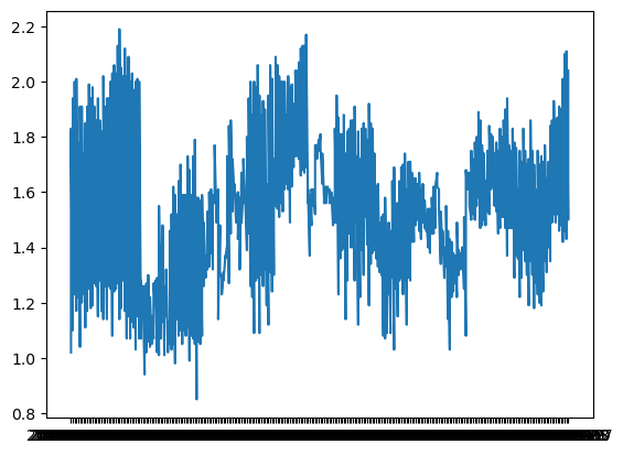
plt.plot(avocados_boston.date, avocados_boston.average_price)
plt.show()

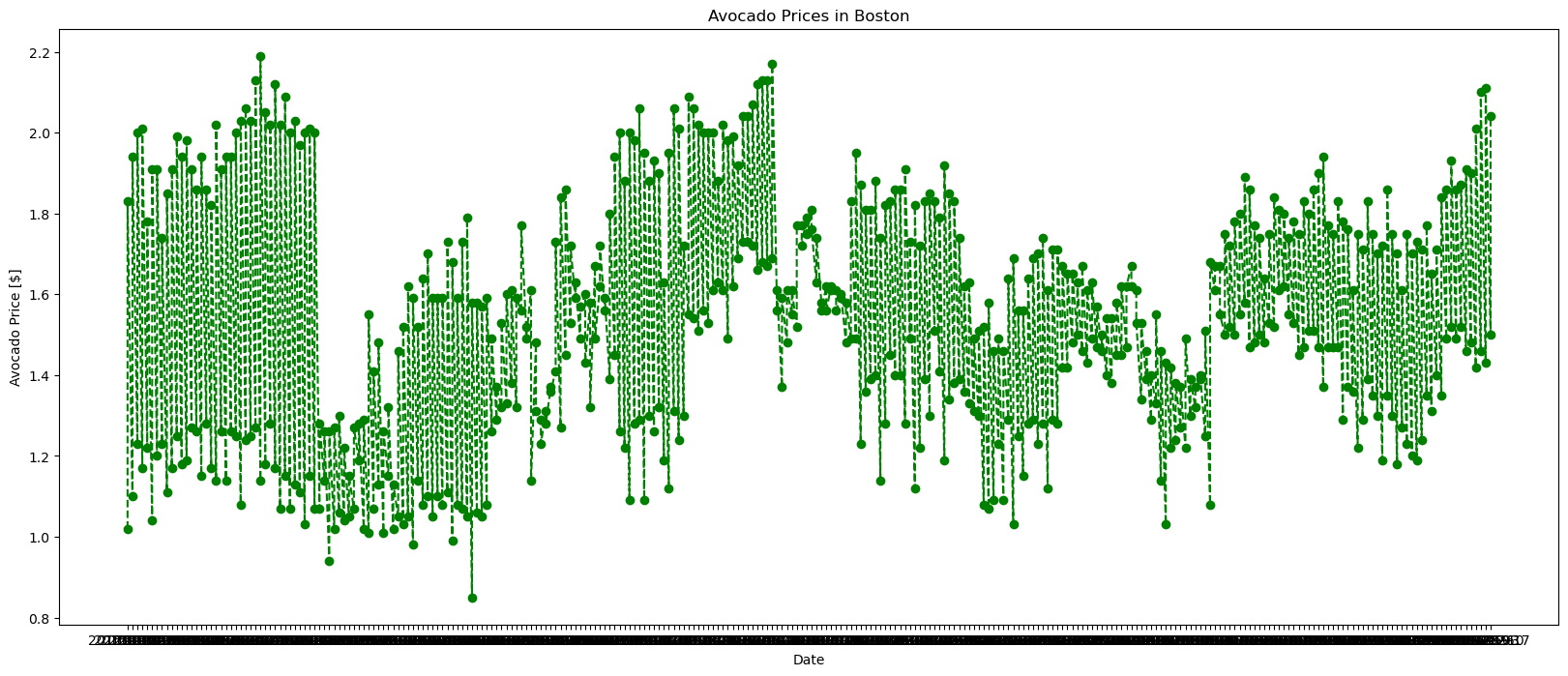
plt.figure(figsize = (20, 8))
plt.plot(avocados_boston.date, avocados_boston.average_price, color = 'green', linestyle = '--', marker = 'o')
plt.xlabel("Date")
plt.ylabel("Avocado Price [$]")
plt.title("Avocado Prices in Boston")
plt.show()

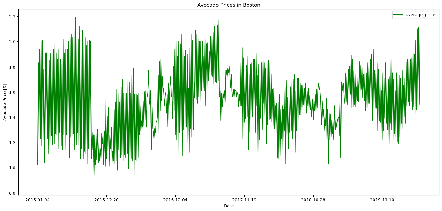
avocados_boston.plot(x = 'date', y = 'average_price', figsize = (18, 8), kind='line', color = 'green')
plt.xlabel("Date")
plt.ylabel("Avocado Price [$]")
plt.title("Avocado Prices in Boston")
plt.show()

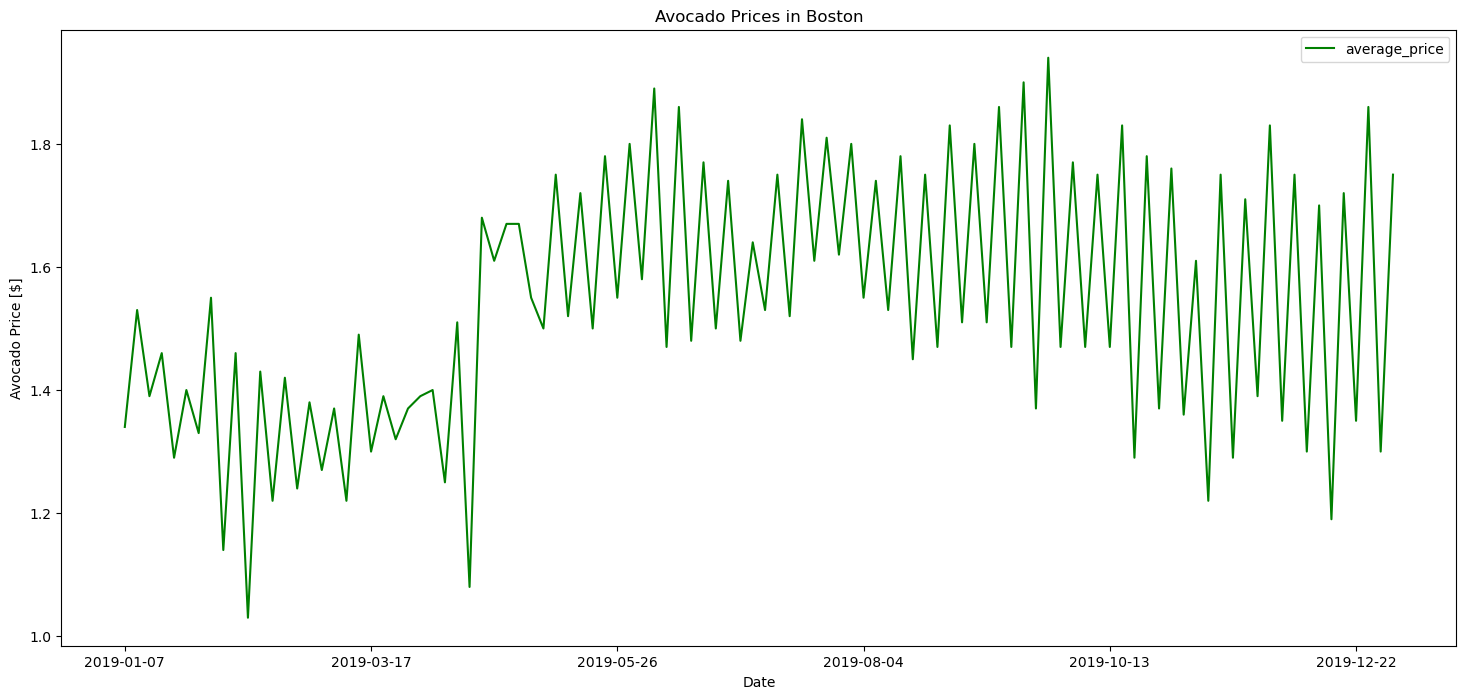
avocados_boston[avocados_boston.year == 2019].plot(x = 'date', y = 'average_price', figsize = (18, 8), kind='line', color = 'green')
plt.xlabel("Date")
plt.ylabel("Avocado Price [$]")
plt.title("Avocado Prices in Boston")
plt.show()

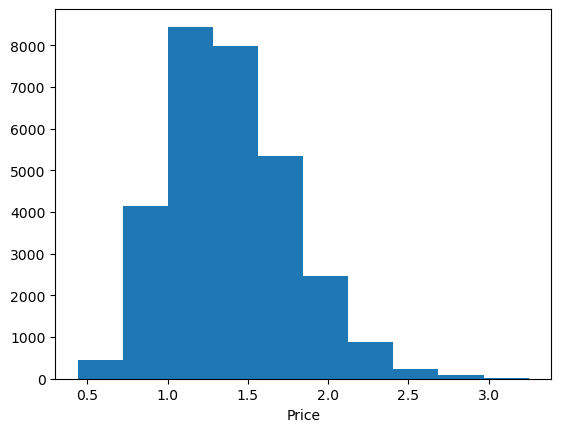
plt.hist(avocados.average_price)
plt.xlabel('Price')
plt.show()

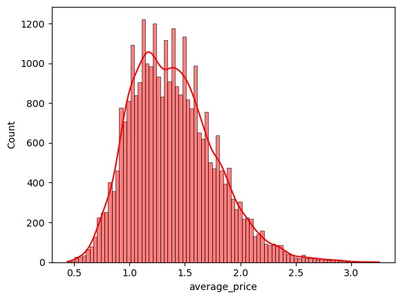
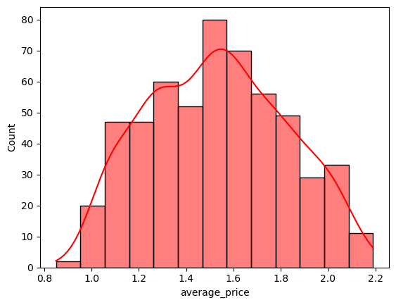
sns.histplot(avocados.average_price, color = 'r', kde = True)

<Axes: xlabel='average_price', ylabel='Count'>

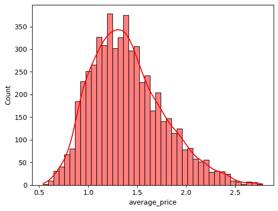
sns.histplot(avocados.average_price[avocados.year == 2019], color = 'r', kde = True)

<Axes: xlabel='average_price', ylabel='Count'>

sns.histplot(avocados.average_price[avocados.geography == 'Boston'], color = 'r', kde = True)

<Axes: xlabel='average_price', ylabel='Count'>

---

Combining Datasets and Long vs Wide Data

pop = pd.read_csv('data/population.csv')

pop

	Country Name	Country Code	Indicator Name	Indicator Code	1960	1961	1962	1963	1964	1965	...	2010	2011	2012	2013	2014	2015	2016	2017	2018	2019
0	Aruba	ABW	Population, total	SP.POP.TOTL	54211.0	55438.0	56225.0	56695.0	57032.0	57360.0	...	101669.0	102046.0	102560.0	103159.0	103774.0	104341.0	104872.0	105366.0	105845.0	106314.0
1	Afghanistan	AFG	Population, total	SP.POP.TOTL	8996973.0	9169410.0	9351441.0	9543205.0	9744781.0	9956320.0	...	29185507.0	30117413.0	31161376.0	32269589.0	33370794.0	34413603.0	35383128.0	36296400.0	37172386.0	38041754.0
2	Angola	AGO	Population, total	SP.POP.TOTL	5454933.0	5531472.0	5608539.0	5679458.0	5735044.0	5770570.0	...	23356246.0	24220661.0	25107931.0	26015780.0	26941779.0	27884381.0	28842484.0	29816748.0	30809762.0	31825295.0
3	Albania	ALB	Population, total	SP.POP.TOTL	1608800.0	1659800.0	1711319.0	1762621.0	1814135.0	1864791.0	...	2913021.0	2905195.0	2900401.0	2895092.0	2889104.0	2880703.0	2876101.0	2873457.0	2866376.0	2854191.0
4	Andorra	AND	Population, total	SP.POP.TOTL	13411.0	14375.0	15370.0	16412.0	17469.0	18549.0	...	84449.0	83747.0	82427.0	80774.0	79213.0	78011.0	77297.0	77001.0	77006.0	77142.0
...	...	...	...	...	...	...	...	...	...	...	...	...	...	...	...	...	...	...	...	...	...
259	Kosovo	XKX	Population, total	SP.POP.TOTL	947000.0	966000.0	994000.0	1022000.0	1050000.0	1078000.0	...	1775680.0	1791000.0	1807106.0	1818117.0	1812771.0	1788196.0	1777557.0	1791003.0	1797085.0	1794248.0
260	Yemen, Rep.	YEM	Population, total	SP.POP.TOTL	5315355.0	5393036.0	5473671.0	5556766.0	5641597.0	5727751.0	...	23154855.0	23807588.0	24473178.0	25147109.0	25823485.0	26497889.0	27168210.0	27834821.0	28498687.0	29161922.0
261	South Africa	ZAF	Population, total	SP.POP.TOTL	17099840.0	17524533.0	17965725.0	18423161.0	18896307.0	19384841.0	...	51216964.0	52004172.0	52834005.0	53689236.0	54545991.0	55386367.0	56203654.0	57000451.0	57779622.0	58558270.0
262	Zambia	ZMB	Population, total	SP.POP.TOTL	3070776.0	3164329.0	3260650.0	3360104.0	3463213.0	3570464.0	...	13605984.0	14023193.0	14465121.0	14926504.0	15399753.0	15879361.0	16363507.0	16853688.0	17351822.0	17861030.0
263	Zimbabwe	ZWE	Population, total	SP.POP.TOTL	3776681.0	3905034.0	4039201.0	4178726.0	4322861.0	4471177.0	...	12697723.0	12894316.0	13115131.0	13350356.0	13586681.0	13814629.0	14030390.0	14236745.0	14439018.0	14645468.0

264 rows × 64 columns

pop.drop(labels = ['Indicator Name', 'Indicator Code'], axis = 1, inplace = True)

pop

	Country Name	Country Code	1960	1961	1962	1963	1964	1965	1966	1967	...	2010	2011	2012	2013	2014	2015	2016	2017	2018	2019
0	Aruba	ABW	54211.0	55438.0	56225.0	56695.0	57032.0	57360.0	57715.0	58055.0	...	101669.0	102046.0	102560.0	103159.0	103774.0	104341.0	104872.0	105366.0	105845.0	106314.0
1	Afghanistan	AFG	8996973.0	9169410.0	9351441.0	9543205.0	9744781.0	9956320.0	10174836.0	10399926.0	...	29185507.0	30117413.0	31161376.0	32269589.0	33370794.0	34413603.0	35383128.0	36296400.0	37172386.0	38041754.0
2	Angola	AGO	5454933.0	5531472.0	5608539.0	5679458.0	5735044.0	5770570.0	5781214.0	5774243.0	...	23356246.0	24220661.0	25107931.0	26015780.0	26941779.0	27884381.0	28842484.0	29816748.0	30809762.0	31825295.0
3	Albania	ALB	1608800.0	1659800.0	1711319.0	1762621.0	1814135.0	1864791.0	1914573.0	1965598.0	...	2913021.0	2905195.0	2900401.0	2895092.0	2889104.0	2880703.0	2876101.0	2873457.0	2866376.0	2854191.0
4	Andorra	AND	13411.0	14375.0	15370.0	16412.0	17469.0	18549.0	19647.0	20758.0	...	84449.0	83747.0	82427.0	80774.0	79213.0	78011.0	77297.0	77001.0	77006.0	77142.0
...	...	...	...	...	...	...	...	...	...	...	...	...	...	...	...	...	...	...	...	...	...
259	Kosovo	XKX	947000.0	966000.0	994000.0	1022000.0	1050000.0	1078000.0	1106000.0	1135000.0	...	1775680.0	1791000.0	1807106.0	1818117.0	1812771.0	1788196.0	1777557.0	1791003.0	1797085.0	1794248.0
260	Yemen, Rep.	YEM	5315355.0	5393036.0	5473671.0	5556766.0	5641597.0	5727751.0	5816247.0	5907874.0	...	23154855.0	23807588.0	24473178.0	25147109.0	25823485.0	26497889.0	27168210.0	27834821.0	28498687.0	29161922.0
261	South Africa	ZAF	17099840.0	17524533.0	17965725.0	18423161.0	18896307.0	19384841.0	19888250.0	20406864.0	...	51216964.0	52004172.0	52834005.0	53689236.0	54545991.0	55386367.0	56203654.0	57000451.0	57779622.0	58558270.0
262	Zambia	ZMB	3070776.0	3164329.0	3260650.0	3360104.0	3463213.0	3570464.0	3681955.0	3797873.0	...	13605984.0	14023193.0	14465121.0	14926504.0	15399753.0	15879361.0	16363507.0	16853688.0	17351822.0	17861030.0
263	Zimbabwe	ZWE	3776681.0	3905034.0	4039201.0	4178726.0	4322861.0	4471177.0	4623351.0	4779827.0	...	12697723.0	12894316.0	13115131.0	13350356.0	13586681.0	13814629.0	14030390.0	14236745.0	14439018.0	14645468.0

264 rows × 62 columns

pop_long = pop.melt(id_vars = ['Country Name', 'Country Code'], var_name = 'Year', value_name = 'Population')

pop_long

	Country Name	Country Code	Year	Population
0	Aruba	ABW	1960	54211.0
1	Afghanistan	AFG	1960	8996973.0
2	Angola	AGO	1960	5454933.0
3	Albania	ALB	1960	1608800.0
4	Andorra	AND	1960	13411.0
...	...	...	...	...
15835	Kosovo	XKX	2019	1794248.0
15836	Yemen, Rep.	YEM	2019	29161922.0
15837	South Africa	ZAF	2019	58558270.0
15838	Zambia	ZMB	2019	17861030.0
15839	Zimbabwe	ZWE	2019	14645468.0

15840 rows × 4 columns

gdp = pd.read_csv('data/gdp.csv').drop(labels = ['Indicator Name', 'Indicator Code'], axis = 1)

gdp

	Country Name	Country Code	1960	1961	1962	1963	1964	1965	1966	1967	...	2010	2011	2012	2013	2014	2015	2016	2017	2018	2019
0	Aruba	ABW	NaN	NaN	NaN	NaN	NaN	NaN	NaN	NaN	...	2.390503e+09	2.549721e+09	2.534637e+09	2.701676e+09	2.765363e+09	2.919553e+09	2.965922e+09	3.056425e+09	NaN	NaN
1	Afghanistan	AFG	5.377778e+08	5.488889e+08	5.466667e+08	7.511112e+08	8.000000e+08	1.006667e+09	1.400000e+09	1.673333e+09	...	1.585657e+10	1.780429e+10	2.000160e+10	2.056107e+10	2.048489e+10	1.990711e+10	1.936264e+10	2.019176e+10	1.948438e+10	1.910135e+10
2	Angola	AGO	NaN	NaN	NaN	NaN	NaN	NaN	NaN	NaN	...	8.379950e+10	1.117900e+11	1.280530e+11	1.367100e+11	1.457120e+11	1.161940e+11	1.011240e+11	1.221240e+11	1.013530e+11	9.463542e+10
3	Albania	ALB	NaN	NaN	NaN	NaN	NaN	NaN	NaN	NaN	...	1.192693e+10	1.289077e+10	1.231983e+10	1.277622e+10	1.322814e+10	1.138685e+10	1.186120e+10	1.301969e+10	1.514702e+10	1.527808e+10
4	Andorra	AND	NaN	NaN	NaN	NaN	NaN	NaN	NaN	NaN	...	3.449967e+09	3.629204e+09	3.188809e+09	3.193704e+09	3.271808e+09	2.789870e+09	2.896679e+09	3.000181e+09	3.218316e+09	3.154058e+09
...	...	...	...	...	...	...	...	...	...	...	...	...	...	...	...	...	...	...	...	...	...
259	Kosovo	XKX	NaN	NaN	NaN	NaN	NaN	NaN	NaN	NaN	...	5.835874e+09	6.701698e+09	6.499807e+09	7.074778e+09	7.396705e+09	6.442916e+09	6.719172e+09	7.245707e+09	7.942962e+09	7.926108e+09
260	Yemen, Rep.	YEM	NaN	NaN	NaN	NaN	NaN	NaN	NaN	NaN	...	3.090675e+10	3.272642e+10	3.540134e+10	4.041524e+10	4.320647e+10	3.697620e+10	2.808468e+10	2.456133e+10	2.759126e+10	NaN
261	South Africa	ZAF	7.575397e+09	7.972997e+09	8.497997e+09	9.423396e+09	1.037400e+10	1.133440e+10	1.235500e+10	1.377739e+10	...	3.753490e+11	4.164190e+11	3.963330e+11	3.668290e+11	3.509050e+11	3.176210e+11	2.963570e+11	3.495540e+11	3.682890e+11	3.514320e+11
262	Zambia	ZMB	7.130000e+08	6.962857e+08	6.931429e+08	7.187143e+08	8.394286e+08	1.082857e+09	1.264286e+09	1.368000e+09	...	2.026556e+10	2.345952e+10	2.550306e+10	2.804551e+10	2.715065e+10	2.124335e+10	2.095476e+10	2.586814e+10	2.700524e+10	2.306472e+10
263	Zimbabwe	ZWE	1.052990e+09	1.096647e+09	1.117602e+09	1.159512e+09	1.217138e+09	1.311436e+09	1.281750e+09	1.397002e+09	...	1.204166e+10	1.410192e+10	1.711485e+10	1.909102e+10	1.949552e+10	1.996312e+10	2.054868e+10	2.204090e+10	2.431156e+10	2.144076e+10

264 rows × 62 columns

gdp_long = gdp.melt(id_vars = ['Country Name', 'Country Code'], var_name = 'Year', value_name = 'GDP')

gdp_long

	Country Name	Country Code	Year	GDP
0	Aruba	ABW	1960	NaN
1	Afghanistan	AFG	1960	5.377778e+08
2	Angola	AGO	1960	NaN
3	Albania	ALB	1960	NaN
4	Andorra	AND	1960	NaN
...	...	...	...	...
15835	Kosovo	XKX	2019	7.926108e+09
15836	Yemen, Rep.	YEM	2019	NaN
15837	South Africa	ZAF	2019	3.514320e+11
15838	Zambia	ZMB	2019	2.306472e+10
15839	Zimbabwe	ZWE	2019	2.144076e+10

15840 rows × 4 columns

countries = pop_long.merge(gdp_long.drop(labels = ['Country Name'], axis = 1), 
                           on = ['Country Code', 'Year'], how = 'inner')

countries

	Country Name	Country Code	Year	Population	GDP
0	Aruba	ABW	1960	54211.0	NaN
1	Afghanistan	AFG	1960	8996973.0	5.377778e+08
2	Angola	AGO	1960	5454933.0	NaN
3	Albania	ALB	1960	1608800.0	NaN
4	Andorra	AND	1960	13411.0	NaN
...	...	...	...	...	...
15835	Kosovo	XKX	2019	1794248.0	7.926108e+09
15836	Yemen, Rep.	YEM	2019	29161922.0	NaN
15837	South Africa	ZAF	2019	58558270.0	3.514320e+11
15838	Zambia	ZMB	2019	17861030.0	2.306472e+10
15839	Zimbabwe	ZWE	2019	14645468.0	2.144076e+10

15840 rows × 5 columns

countries['GDP per capita'] = countries['GDP'] / countries['Population']

countries

	Country Name	Country Code	Year	Population	GDP	GDP per capita
0	Aruba	ABW	1960	54211.0	NaN	NaN
1	Afghanistan	AFG	1960	8996973.0	5.377778e+08	59.773194
2	Angola	AGO	1960	5454933.0	NaN	NaN
3	Albania	ALB	1960	1608800.0	NaN	NaN
4	Andorra	AND	1960	13411.0	NaN	NaN
...	...	...	...	...	...	...
15835	Kosovo	XKX	2019	1794248.0	7.926108e+09	4417.509940
15836	Yemen, Rep.	YEM	2019	29161922.0	NaN	NaN
15837	South Africa	ZAF	2019	58558270.0	3.514320e+11	6001.406804
15838	Zambia	ZMB	2019	17861030.0	2.306472e+10	1291.343357
15839	Zimbabwe	ZWE	2019	14645468.0	2.144076e+10	1463.985910

15840 rows × 6 columns

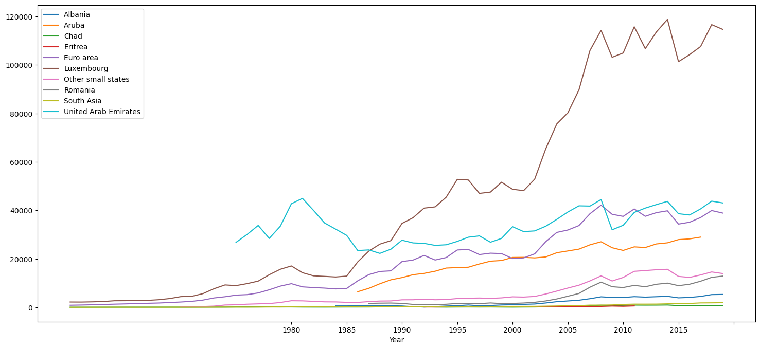
random_countries = np.random.choice(countries['Country Code'].unique(), 10)

countries_select = countries[countries['Country Code'].isin(random_countries)]

countries_select

	Country Name	Country Code	Year	Population	GDP	GDP per capita
0	Aruba	ABW	1960	5.421100e+04	NaN	NaN
3	Albania	ALB	1960	1.608800e+06	NaN	NaN
6	United Arab Emirates	ARE	1960	9.241800e+04	NaN	NaN
66	Euro area	EMU	1960	2.652039e+08	2.448960e+11	923.425216
67	Eritrea	ERI	1960	1.007590e+06	NaN	NaN
...	...	...	...	...	...	...
15718	Luxembourg	LUX	2019	6.198960e+05	7.110492e+10	114704.594171
15757	Other small states	OSS	2019	3.136041e+07	4.384680e+11	13981.578747
15775	Romania	ROU	2019	1.935654e+07	2.500770e+11	12919.506705
15778	South Asia	SAS	2019	1.835777e+09	3.597970e+12	1959.916976
15803	Chad	TCD	2019	1.594688e+07	1.131495e+10	709.540310

600 rows × 6 columns

for name, data in countries_select.groupby('Country Name'):
    data.plot(x = 'Year', y = 'GDP per capita', label = name, figsize = (18, 8), ax = plt.gca())
plt.show()